
Production scrap is the material and finished parts you discard because they fail specification, and you reduce it by finding the few critical variables (in the material, the process and the incoming inputs) that cause most of the rejection, then measuring them and holding them under statistical control before they eat your margin.
PROCESS IMPROVEMENT
Do you want to reduce scrap and waste in your production? Discover our process improvement service

What scrap is and why it eats your margin
Scrap is any unit you produce that you cannot sell or use, and that you therefore discard or downgrade below the value you had planned for it. It covers parts outside tolerance, contaminated material, lots rejected at quality control and reworked product that no longer reaches the original specification. Every one of those units has already absorbed material, energy, machine time and labour before it became a loss, and that is precisely why scrap weighs far more than its “waste” label suggests.
On an industrial P&L, scrap rarely shows up under its own name. It hides inside the price of the lost material, the hours of rework, the energy burned on parts that end up in the skip and the orders that ship late. Treating that rejection as an unavoidable constant is an expensive decision, because most scrap concentrates in a handful of causes, and going after them in an orderly way is exactly the territory of process improvement, one of the central levers of materials innovation.
The most common management mistake is to count only the material thrown away and consider the calculation closed. A defect that keeps repeating (a burr, a surface mark, a dimension that drifts) does not cost you just the part: it costs the extra inspection you are forced to set up, the rework, the returns and, at times, the customer’s confidence. Take an analysis of aesthetic defects that were causing rejects in electronic components, which shows how far an apparently cosmetic problem can push up both the rejection rate and the cost attached to it.
The direct cost of scrap: material that leaves the line and never comes back
The direct cost of scrap is the value of the material and the built-in labour you lose for good the moment a part is discarded. It climbs with every operation: a steel bar scrapped before machining costs you only the price of the material, but that same part rejected after machining, heat treatment and coating already drags the cost of all those stages with it. In a foundry, a casting rejected for porosity after finish machining has swallowed melt energy, mould material, machine time and inspection before it is even flagged. That is why scrap caught late is far more expensive than scrap caught early: throwing away raw material is not the same as throwing away an almost finished part.
This cumulative effect has a direct practical consequence. The point on the line where you catch the defect matters as much as the defect itself. If the rejection turns up at final inspection, you have already paid for the whole process; if you catch it at the operation that generates it, you cap the loss at what you had invested up to that point. Measuring scrap by stage, and not just the total at the end of the shift, is the first step to knowing what it truly costs you and where it is being generated.
The hidden costs of scrap are every expense the rejection triggers without ever appearing under the “discarded material” line: rework, additional inspection, machine and staff time, energy, line stoppages to readjust, delivery delays and contractual penalties. In many processes they exceed the direct cost of the material, and they are what turn a supposedly “acceptable” scrap percentage into a margin leak that is hard to trace. A rework loop, in particular, is deceptive: the part is eventually shipped, so it never registers as scrap, yet it has consumed a second pass of labour, energy and capacity that no one costed.
There is also an opportunity cost that rarely gets logged. Every hour a machine spends producing, inspecting or reworking parts that will end up discarded is capacity you are not devoting to sellable product. When the plant is tight on capacity, scrap does not only cost money, it also caps what you can invoice. That is why “a bit of scrap” is not an unavoidable toll of manufacturing: it is a problem with concrete causes that, once identified, can be controlled. When the same defect reappears shift after shift, the profitable move is identifying the cause of a repetitive failure in production instead of continuing to absorb it as a fixed cost.
The hidden costs of scrap (rework, extra inspection, a stopped line, energy and penalties) usually outweigh the discarded material itself. Counting only the part you threw away understates the problem, and it explains why a seemingly small rejection rate can erode a large share of a product’s margin.
Where the critical variables of scrap come from
The critical variables of scrap are the few factors (in the material, the process and the inputs) that, when they drift, cause most of a line’s rejection. Not every variable in a process carries the same weight: following the Pareto principle, a minority concentrates the majority of the defects, and finding them is what lets you reduce scrap without redesigning the whole operation. Rigorous characterisation of the material and the process is what separates those underlying variables from everyday noise.
It helps to sort the origin into three families. The first is the material coming through the door: each lot arrives with its own variability in composition, microstructure or mechanical properties, and that variability transfers to the part. The second is the parameters of the process itself (temperature, pressure, speed, tooling wear). The third is the design and the tolerances the part is specified with. On most lines, the bulk of the scrap comes from one or two variables within these families, not from a diffuse problem spread evenly everywhere at once.
Material and batch variability: when scrap comes in from the supplier
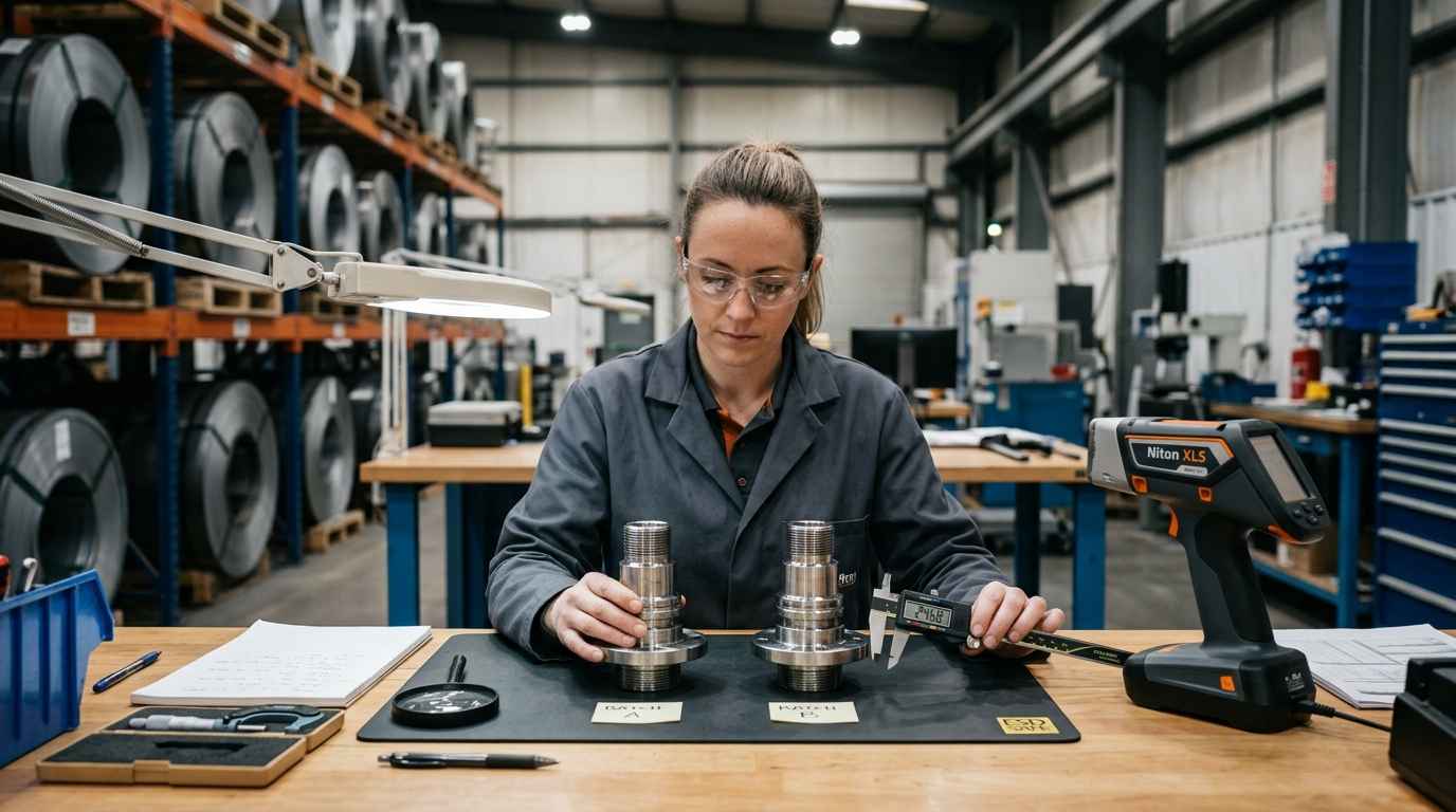
Material variability is the first source of scrap because it introduces differences the process cannot always compensate for. Two lots of the same reference can both meet the supplier’s certificate and still behave differently on the line: a hardness at the top of the range, a slightly shifted composition or a different microstructure change how the material flows, forms or machines, and that shows up as defects that appear “for no obvious reason” right when you switch lots. A steel coil at the hard end of its band can crack in a deep-draw press that ran clean for months.
When scrap spikes after a change of coil, heat or supplier, the critical variable is not in the machine, it is in the input. Confirming it means measuring the material, not assuming it: an alloy composition analysis reveals whether a lot has drifted out of range, and comparing properties between good and bad lots isolates which material characteristic correlates with the rejection. That comparison also builds the evidence you need to take back to the supplier, while an analysis of metal needles in anomalous production batches illustrates how a material anomaly is traced back to the specific lot that introduced it.
Reducing scrap is not about watching everything, but about finding the critical variables that concentrate most of the rejection. The Pareto principle holds stubbornly in manufacturing: a few material and process factors explain the majority of the parts that end up discarded, and they are what you go after first.
Process parameters, design and tolerances: the Pareto principle applied to scrap
Process parameters become critical variables when their drift or their spread pushes the part out of tolerance in a systematic way. An injection temperature that fluctuates, a holding pressure that drops at the end of the shift, tooling that wears or a badly set feed rate generate recurring defects (flash, sink marks, burrs, surface finish out of spec) that do not depend on the operator but on the setting and the stability of the process. Identifying which of those parameters genuinely move the result, and which are irrelevant, is the core of scrap reduction, because tightening a parameter that has no effect only adds cost and slows the line.
Design and tolerances close the triangle. A dimension with a tolerance tighter than the process can hold generates scrap by definition, even when everything is running “well”: the process is simply not capable of meeting what the drawing demands. In those cases the critical variable is neither in the material nor in the machine, but in a design requirement too demanding for the real capability, and the fix runs through reviewing the tolerance or the product itself via product improvement, not through squeezing a process that is already at its limit.
TELL US ABOUT YOUR CASE
Do you have a process with too much scrap? Send us your case and we will propose an analysis of the critical variables
How to find and control the critical variables
Finding the critical variables of scrap means moving from opinion to data: measuring the process and the material, reconstructing the root-cause chain and checking with evidence which factors move the rejection. The usual sequence links four steps (measure and classify the scrap, analyse the root cause, characterise the material involved and control the confirmed variables), and each one leans on concrete tools. Material characterisation supplies the objective part when the suspicion points at the raw material rather than the equipment.
Before you change anything, it helps to have the map. The table below summarises the three families of critical variables, how each one shows up as scrap and the tools you use to identify and control it.
| Type of critical variable | How it shows up as scrap | How it is identified and controlled |
|---|---|---|
| Material and lot (input) | Defects that appear when you change lot, heat or supplier despite the certificate being in order | Material characterisation and composition analysis; comparison between good and bad lots; a stricter incoming specification |
| Process parameters | Recurring rejection from drift or spread (temperature, pressure, speed, tooling wear) | Statistical process control (SPC), Cp/Cpk capability studies and design of experiments (DOE) to set the optimal parameters |
| Design and tolerances | Parts out of dimension even with a stable process: the tolerance asks for more than the process can give | Capability study against the tolerance; review of the dimension or the design (product improvement) to match real capability |
| Diffuse root cause | Intermittent defect with no clear pattern and several candidate causes at once | Structured root cause analysis (8D, Ishikawa diagram, FMEA) to separate the real cause from the noise |
With that map in front of you, start where the loss is largest. Pull your scrap records by defect and by stage before you touch a single parameter, and the work then splits into two fronts: finding the cause when the defect is elusive, and controlling the variable once you know which one it is.
Root cause analysis of scrap: 8D, Ishikawa and FMEA
Root cause analysis is the structured method that leads from an observed defect to the variable that causes it, without stopping at the symptom. The 8D (eight disciplines) organises team problem-solving, from immediate containment of the defect through to a verified corrective action; the Ishikawa (or cause-effect) diagram sorts the possible causes into families (material, machine, method, labour, measurement, environment) so that none is left unchecked; and FMEA (failure mode and effects analysis) ranks the causes by their severity, their frequency and how easy they are to detect, so you attack the ones that matter first.
These tools do not find the cause on their own: the data they organise does. That is why they work when you combine them with the physical evidence of the defect (the rejected part, the material, the process record) rather than with a meeting-room hypothesis. When the defect is recurring and its origin is unclear, a failure analysis adds the forensic part (fractography, microscopy and material analysis) that confirms or rules out each hypothesis instead of leaving it to judgement. That way you avoid the usual and expensive mistake of “correcting” a cause that was not the real one and carrying on generating scrap.
Root cause analysis with 8D, Ishikawa and FMEA does not replace measurement: it orders it. These methodologies structure the hypotheses, but it is the physical evidence from the material and the process that confirms which of those variables is actually generating the scrap.
SPC, process capability (Cp/Cpk) and DOE to control scrap
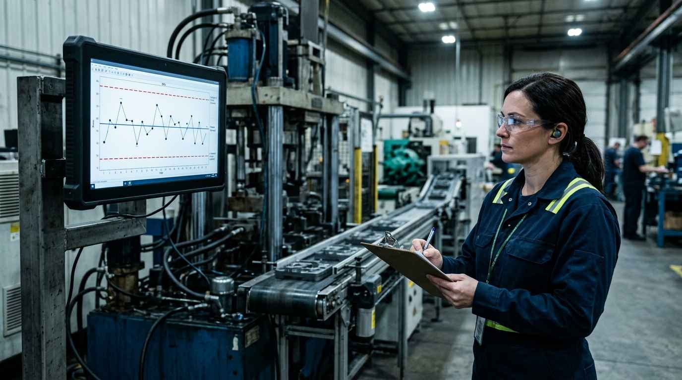
Once you have identified the critical variable, controlling it means keeping it inside a range the process can hold in a stable way, and that is where three complementary tools come in. Statistical process control (SPC) watches the variable in real time with control charts and tells the normal variation of the process apart from a real deviation you need to correct, so you react to signals and not to noise. Process capability studies (the Cp and Cpk indices) then compare the spread of the process against the tolerance limits and quantify how much scrap you should expect: a low Cpk anticipates rejection even when the process is perfectly centred, because the natural variation alone is wider than the tolerance allows.
Design of experiments (DOE) closes the loop when several variables are in play and it is not clear which one weighs most. Instead of changing one parameter at a time, DOE varies several of them in a planned way to measure their individual effect and their interactions, and it returns the settings that minimise rejection with the fewest trials. Consolidating these controls (SPC to watch, Cp/Cpk to verify capability, DOE to optimise) inside the quality management system, within the ISO 9001 continual-improvement framework, is what turns a one-off correction into a scrap reduction that holds shift after shift.
Reducing scrap in production stops being a constant battle once you control the few variables that concentrate it: statistical process control and the Cp/Cpk capability indices anticipate rejection before it happens and turn scrap from a recurring surprise into a predictable, manageable variable.
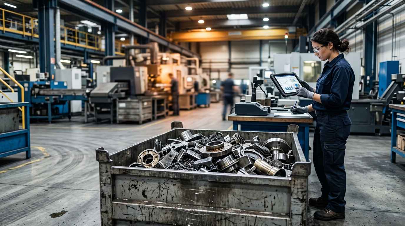
Turning scrap into a margin lever, not a toll you pay
Reducing scrap in production is not about chasing every bad part, but about identifying the few material, process and design variables that concentrate most of the rejection and bringing them under control. The cost of scrap does not end at the discarded material: it includes rework, inspection, energy, lost capacity and lead times, and that is why every point of rejection you eliminate shows up in the margin far more than the price of the part would ever suggest.
The sequence that works is always the same. Measure scrap by stage and by defect so you know where and how much you lose, use root cause analysis to reach the real variable instead of the symptom, characterise the material when the suspicion points at the input, and control the confirmed variables with SPC, process capability and design of experiments. That order turns a diffuse problem into a manageable number of variables, and scrap stops being a toll you accept and becomes a margin lever you decide on.
If your line carries a rejection rate that nobody questions any more and you are not sure what is driving it, gather what you already have to hand (the scrap records by defect and by stage, the material lots involved, the process parameters and a few representative rejected parts) and put the case to us. From that starting point, INFINITIA characterises the material, reconstructs the root-cause chain and tells you which few variables concentrate your scrap and how to keep them under control. Write to us, describe your recurring defect and define with us the first experiment that separates the real cause from the noise.
Frequently asked questions about reducing production scrap
What is production scrap and how do you calculate its cost?
Production scrap is the material and parts you discard because they fail specification, and its real cost is calculated by adding the lost material, the labour and energy already built in, the rework, the additional inspection and the effects of lead time or penalties. Costing it only by the value of the discarded material understates the problem, because most of the cost usually sits in the hidden costs (rework, a stopped line and lost capacity). Measuring scrap by stage lets you see how much it costs depending on the point at which you catch it.
How do you identify the critical variables that generate scrap?
The critical variables are identified by measuring the process and the material and applying root cause analysis to separate the few causes that concentrate most of the rejection. In practice you combine the scrap record by defect and by stage, tools such as 8D, the Ishikawa diagram and FMEA to order the hypotheses, and the comparison of data between good and bad lots or conditions. The aim is to confirm with evidence which factor moves the rejection, not to assume it from experience.
Why is controlling the process not enough if the problem comes from the material?
When the critical variable sits in the incoming material, adjusting the process only masks the problem and consumes capacity without eliminating the scrap. If a lot arrives with a shifted composition or shifted properties, the part will come out defective even with the machine perfectly set. Confirming the origin means measuring the material (for example, with composition analysis and characterisation) and, where appropriate, tightening the incoming specification so that variability never makes it onto the line in the first place.
What is process capability (Cp/Cpk) and how does it relate to scrap?
Process capability is the relationship between the natural spread of a process and the tolerance limits of the part, quantified with the Cp and Cpk indices. A high Cpk means the process runs comfortably within tolerance and generates little rejection; a low Cpk anticipates scrap even before an incident occurs, because the variation approaches or exceeds the limits. That is why a capability study lets you predict and prevent scrap instead of reacting to it after the parts are already in the bin.
How long does an analysis to find the cause of scrap take?
An analysis to locate the cause of scrap usually takes between one and four weeks depending on the complexity of the defect and the number of variables involved, with an urgent option in 24 to 72 hours for cases that have the line stopped. The timescale depends on whether the material needs to be characterised, the defect reproduced or data across several lots correlated. Send a description of the defect, the lots involved and representative parts to scope the work and estimate the real time.